
实例介绍
【实例简介】逻辑回归与分类
【实例截图】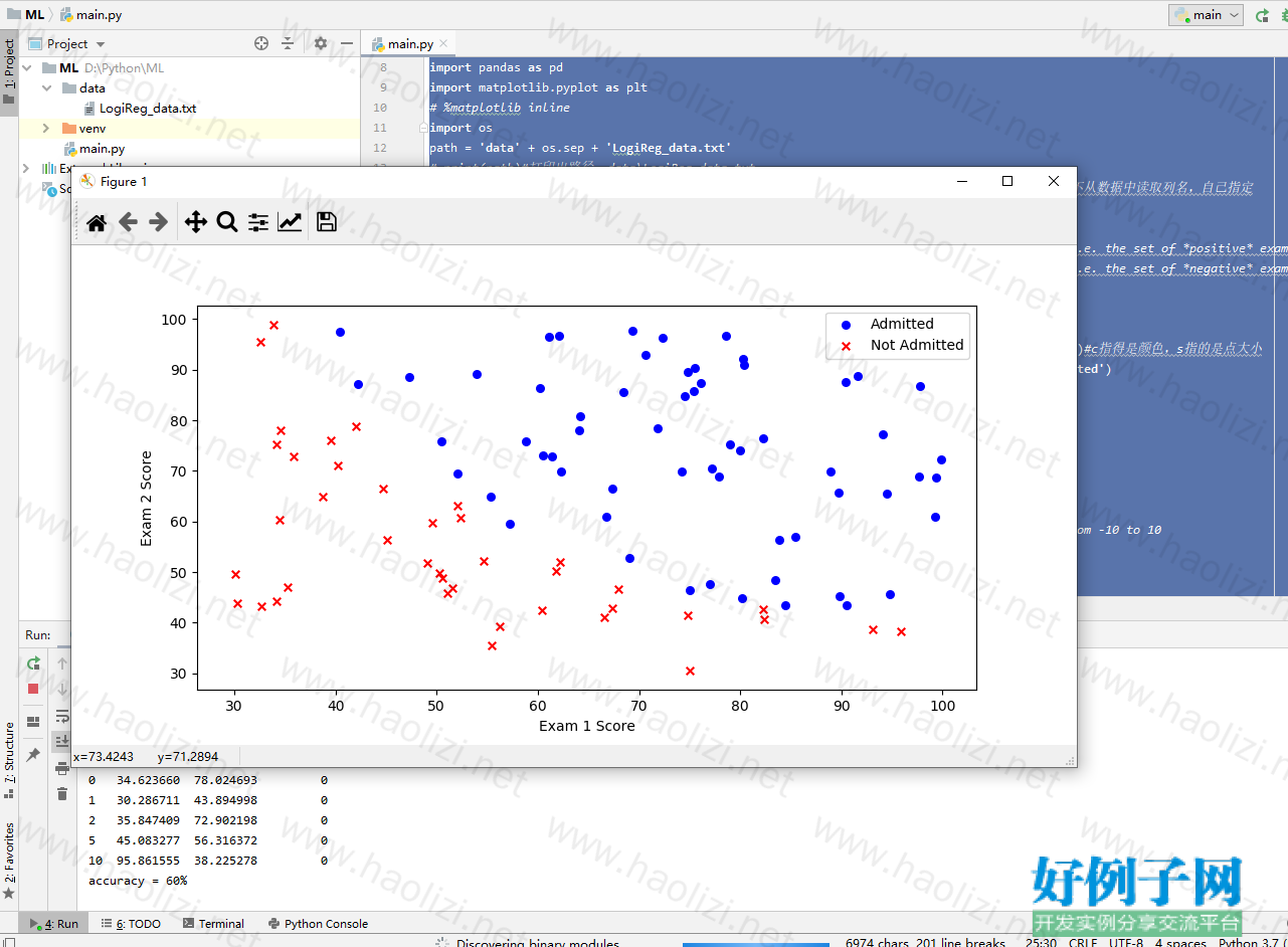
【核心代码】
【实例截图】
【核心代码】
# This is a sample Python script.  # Press Shift F10 to execute it or replace it with your code. # Press Double Shift to search everywhere for classes, files, tool windows, actions, and settings.   import numpy as np import pandas as pd import matplotlib.pyplot as plt # %matplotlib inline import os
path = 'data'  os.sep 'LogiReg_data.txt' # print(path)#打印出路径 data\LogiReg_data.txt pdData = pd.read_csv(path, header=None, names=['Exam 1', 'Exam 2', 'Admitted'])#header=None不从数据中读取列名,自己指定 pdData.head()
pdData.shape#查看数据维度 (100, 3) positive = pdData[pdData['Admitted'] == 1] # returns the subset of rows such Admitted = 1, i.e. the set of *positive* examples negative = pdData[pdData['Admitted'] == 0] # returns the subset of rows such Admitted = 0, i.e. the set of *negative* examples print(positive.head())
print(negative.head())
fig, ax = plt.subplots(figsize=(10,5))#设置图的大小 ax.scatter(positive['Exam 1'], positive['Exam 2'], s=30, c='b', marker='o', label='Admitted')#c指得是颜色,s指的是点大小 ax.scatter(negative['Exam 1'], negative['Exam 2'], s=30, c='r', marker='x', label='Not Admitted')
ax.legend()
ax.set_xlabel('Exam 1 Score')
ax.set_ylabel('Exam 2 Score') def sigmoid(z): return 1 / (1  np.exp(-z)) # nums = np.arange(-10, 10, step=1) #creates a vector containing 20 equally spaced values from -10 to 10 # fig, ax = plt.subplots(figsize=(12,4)) # ax.plot(nums, sigmoid(nums), 'r')   def model(X, theta): return sigmoid(np.dot(X, theta.T))
pdData.insert(0, 'Ones', 1) # in a try / except structure so as not to return an error if the block si executed several times #增加一个全1的列 # print(pdData.head()) # set X (training data) and y (target variable)   #orig_data = pdData.as_matrix() # convert the Pandas representation of the data to an array useful for further computations orig_data = pdData.values #print(orig_data) cols = orig_data.shape[1] #print(cols)#4 X = orig_data[:,0:cols-1] #print(X) y = orig_data[:,cols-1:cols] #print(y) # convert to numpy arrays and initalize the parameter array theta #X = np.matrix(X.values) #y = np.matrix(data.iloc[:,3:4].values) #np.array(y.values) theta = np.zeros([1, 3]) #print(theta)  def cost(X, y, theta):
    left = np.multiply(-y, np.log(model(X, theta)))
    right = np.multiply(1 - y, np.log(1 - model(X, theta))) return np.sum(left - right) / (len(X))
cost(X, y, theta)#0.69314718055994529   def gradient(X, y, theta):
    grad = np.zeros(theta.shape)
    error = (model(X, theta) - y).ravel() for j in range(len(theta.ravel())): # for each parmeter  term = np.multiply(error, X[:, j])
        grad[0, j] = np.sum(term) / len(X) return grad
STOP_ITER = 0#迭代次数标志 STOP_COST = 1#损失标志    即两次迭代目标函数之间的差异 STOP_GRAD = 2#梯度变化标志 #以上为三种停止策略,分别是按迭代次数、按损失函数的变化量、按梯度变化量 def stopCriterion(type, value, threshold):#thershold为指定阈值  #设定三种不同的停止策略  if type == STOP_ITER: return value > threshold#按迭代次数停止  elif type == STOP_COST: return abs(value[-1]-value[-2]) < threshold#按损失函数是否改变停止  elif type == STOP_GRAD: return np.linalg.norm(value) < threshold#按梯度大小停止  import numpy.random # 洗牌 def shuffleData(data):
    np.random.shuffle(data)
    cols = data.shape[1]
    X = data[:, 0:cols - 1]
    y = data[:, cols - 1:] return X, y import time def descent(data, theta, batchSize, stopType, thresh, alpha): # 最主要函数:梯度下降求解 batchSize:为1代表随机梯度下降,为整体值表示批量梯度下降,为某一数值表示小批量梯度下降  # stopType:停止策略类型 thresh阈值 alpha学习率  init_time = time.time()
    i = 0 # 迭代次数  k = 0 # batch 迭代数据的初始量  X, y = shuffleData(data)
    grad = np.zeros(theta.shape) # 计算的梯度  costs = [cost(X, y, theta)] # 损失值   while True:
        grad = gradient(X[k:k   batchSize], y[k:k   batchSize], theta) # batchSize为指定的梯度下降策略  k  = batchSize # 取batch数量个数据  if k >= n:
            k = 0  X, y = shuffleData(data) # 重新洗牌  theta = theta - alpha * grad # 参数更新  costs.append(cost(X, y, theta)) # 计算新的损失  i  = 1   if stopType == STOP_ITER:
            value = i elif stopType == STOP_COST:
            value = costs elif stopType == STOP_GRAD:
            value = grad if stopCriterion(stopType, value, thresh): break   return theta, i - 1, costs, grad, time.time() - init_time def runExpe(data, theta, batchSize, stopType, thresh, alpha):#损失率与迭代次数的展示函数  #import pdb; pdb.set_trace();  theta, iter, costs, grad, dur = descent(data, theta, batchSize, stopType, thresh, alpha)
    name = "Original" if (data[:,1]>2).sum() > 1 else "Scaled"  name  = " data - learning rate: {} - ".format(alpha) if batchSize==n: strDescType = "Gradient"  elif batchSize==1:  strDescType = "Stochastic"  else: strDescType = "Mini-batch ({})".format(batchSize)
    name  = strDescType " descent - Stop: "  if stopType == STOP_ITER: strStop = "{} iterations".format(thresh) elif stopType == STOP_COST: strStop = "costs change < {}".format(thresh) else: strStop = "gradient norm < {}".format(thresh)
    name  = strStop
    print ("***{}\nTheta: {} - Iter: {} - Last cost: {:03.2f} - Duration: {:03.2f}s".format(
        name, theta, iter, costs[-1], dur))
    fig, ax = plt.subplots(figsize=(12,4))
    ax.plot(np.arange(len(costs)), costs, 'r')
    ax.set_xlabel('Iterations')
    ax.set_ylabel('Cost')
    ax.set_title(name.upper() ' - Error vs. Iteration') return theta #选择的梯度下降方法是基于所有样本的 n=100#数据样本就100个  # runExpe(orig_data, theta, 100, STOP_ITER, thresh=5000, alpha=0.000001) # runExpe(orig_data, theta, 100, STOP_COST, thresh=0.000001, alpha=0.001) # runExpe(orig_data, theta, 100, STOP_GRAD, thresh=0.05, alpha=0.001)  # runExpe(orig_data, theta, 1, STOP_ITER, thresh=5000, alpha=0.001)  # 1指的是每次只迭代1个样本 # runExpe(orig_data, theta, 1, STOP_ITER, thresh=15000, alpha=0.000002)  # runExpe(orig_data, theta, 16, STOP_ITER, thresh=15000, alpha=0.001)#16指的是每次只迭代16个样本 # runExpe(orig_data, theta, 16, STOP_ITER, thresh=15000, alpha=0.00001)  ##BN from sklearn import preprocessing as pp
scaled_data = orig_data.copy()
scaled_data[:, 1:3] = pp.scale(orig_data[:, 1:3]) # print(scaled_data[:, 1:3])  # runExpe(scaled_data, theta, 100, STOP_ITER, thresh=5000, alpha=0.001) # runExpe(scaled_data, theta, 16, STOP_GRAD, thresh=0.02, alpha=0.001) # theta = runExpe(scaled_data, theta, 1, STOP_GRAD, thresh=0.02/5, alpha=0.001)  #设定阈值 def predict(X, theta): return [1 if x >= 0.5 else 0 for x in model(X, theta)] ##test scaled_X = scaled_data[:, :3]
y = scaled_data[:, 3]
predictions = predict(scaled_X, theta)
correct = [1 if ((a == 1 and b == 1) or (a == 0 and b == 0)) else 0 for (a, b) in zip(predictions, y)]
accuracy = (sum(map(int, correct)) % len(correct))
print ('accuracy = {0}%'.format(accuracy)) # print(theta) # x_new=[1, 80, 60] # print(x_new) # y_value=np.dot(theta, x_new) # y_new=predict(x_new, theta) # print(y_value) # print(y_new)  # x2_mean=65.6442740573232 # x2_std=19.3606867124761 # x3_mean=66.2219980881170 # x3_std=18.4896356705888 # xj=(xj-mean)/std  plt.show()
好例子网口号:伸出你的我的手 — 分享!
相关软件
小贴士
感谢您为本站写下的评论,您的评论对其它用户来说具有重要的参考价值,所以请认真填写。
- 类似“顶”、“沙发”之类没有营养的文字,对勤劳贡献的楼主来说是令人沮丧的反馈信息。
- 相信您也不想看到一排文字/表情墙,所以请不要反馈意义不大的重复字符,也请尽量不要纯表情的回复。
- 提问之前请再仔细看一遍楼主的说明,或许是您遗漏了。
- 请勿到处挖坑绊人、招贴广告。既占空间让人厌烦,又没人会搭理,于人于己都无利。
关于好例子网
本站旨在为广大IT学习爱好者提供一个非营利性互相学习交流分享平台。本站所有资源都可以被免费获取学习研究。本站资源来自网友分享,对搜索内容的合法性不具有预见性、识别性、控制性,仅供学习研究,请务必在下载后24小时内给予删除,不得用于其他任何用途,否则后果自负。基于互联网的特殊性,平台无法对用户传输的作品、信息、内容的权属或合法性、安全性、合规性、真实性、科学性、完整权、有效性等进行实质审查;无论平台是否已进行审查,用户均应自行承担因其传输的作品、信息、内容而可能或已经产生的侵权或权属纠纷等法律责任。本站所有资源不代表本站的观点或立场,基于网友分享,根据中国法律《信息网络传播权保护条例》第二十二与二十三条之规定,若资源存在侵权或相关问题请联系本站客服人员,点此联系我们。关于更多版权及免责申明参见 版权及免责申明

网友评论
我要评论